Efficient Sampling

Importance Sampling via Transmittance Estimator.

Efficient sampling is a well-explored problem in Graphics, wherein the emphasis is on identifying regions that make the most significant contribution to the final rendering. This objective is generally accomplished through importance sampling, which aims to distribute samples based on the probability density function (PDF), denoted as \(p(t)\), between the range of \([t_n, t_f]\). By computing the cumulative distribution function (CDF) through integration, i.e., \(F(t) = \int_{t_n}^{t} p(v)\,dv\), samples are generated using the inverse transform sampling method:

\[t = F^{-1}(u) \quad \text{where} \quad u \sim \mathcal{U}[0,1].\]

In volumetric rendering, the contribution of each sample to the final rendering is expressed by the accumulation weights \(T(t)\sigma(t)\):

\[C(\mathbf{r}) = \int_{t_n}^{t_f} T(t)\,\sigma(t)\,c(t)\,dt\]

Hence, the PDF for volumetric rendering is \(p(t) = T(t)\sigma(t)\) and the CDF is:

\[F(t) = \int_{t_n}^{t} T(v)\sigma(v)\,dv = 1 - T(t)\]

Therefore, inverse sampling the CDF \(F(t)\) is equivalent to inverse sampling the transmittance \(T(t)\). A transmittance estimator is sufficient to determine the optimal samples. We refer readers to the SIGGRAPH 2017 Course: Production Volume Rendering for more details about this concept if within interests.

Occupancy Grid Estimator.

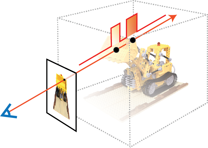
The idea of Occupancy Grid is to cache the density in the scene with a binaraized voxel grid. When sampling, the ray marches through the grid with a preset step sizes, and skip the empty regions by querying the voxel grid. Intuitively, the binaraized voxel grid is an estimator of the radiance field, with much faster readout. This technique is proposed in Instant-NGP with highly optimized CUDA implementations. More formally, The estimator describes a binaraized density distribution \(\hat{\sigma}\) along the ray with a conservative threshold \(\tau\):

\[\hat{\sigma}(t_i) = \mathbb{1}\big[\sigma(t_i) > \tau\big]\]

Consequently, the piece-wise constant PDF can be expressed as

\[p(t_i) = \hat{\sigma}(t_i) / \sum_{j=1}^{n} \hat{\sigma}(t_j)\]

and the piece-wise linear transmittance estimator is

\[T(t_i) = 1 - \sum_{j=1}^{i-1}\hat{\sigma}(t_j) / \sum_{j=1}^{n} \hat{\sigma}(t_j)\]

See the figure below for an illustration.

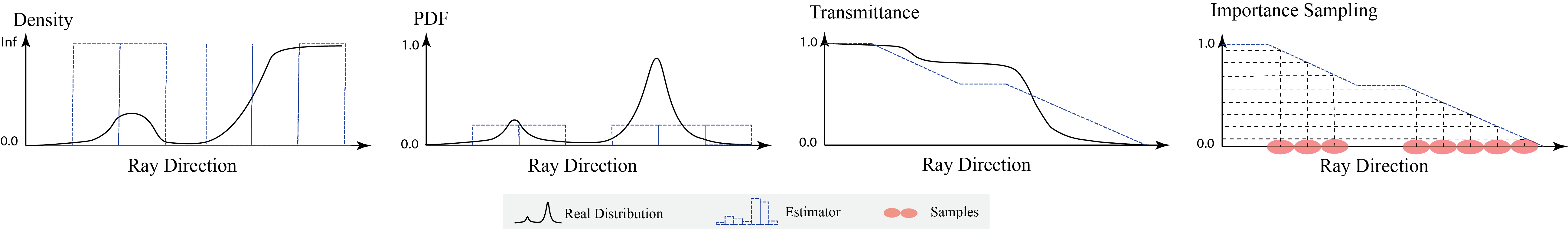
In nerfacc, this is implemented via the nerfacc.OccGridEstimator class.

Proposal Network Estimator.

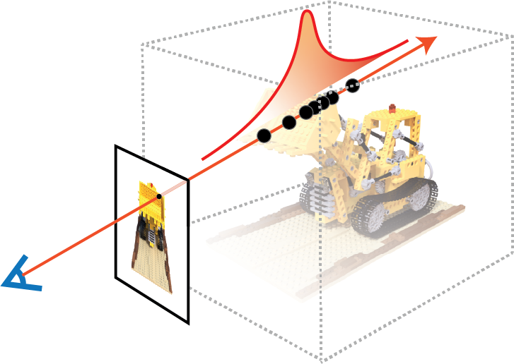
Another type of approach is to directly estimate the PDF along the ray with discrete samples. In vanilla NeRF, the coarse MLP is trained using volumetric rendering loss to output a set of densities \({\sigma(t_i)}\). This allows for the creation of a piece-wise constant PDF:

\[p(t_i) = \sigma(t_i)\exp(-\sigma(t_i)\,dt)\]

and a piece-wise linear transmittance estimator:

\[T(t_i) = \exp(-\sum_{j=1}^{i-1}\sigma(t_i)\,dt)\]

This approach was further improved in Mip-NeRF 360 with a PDF matching loss, which allows for the use of a much smaller MLP in the coarse level, namely Proposal Network, to speedup the PDF construction.

See the figure below for an illustration.

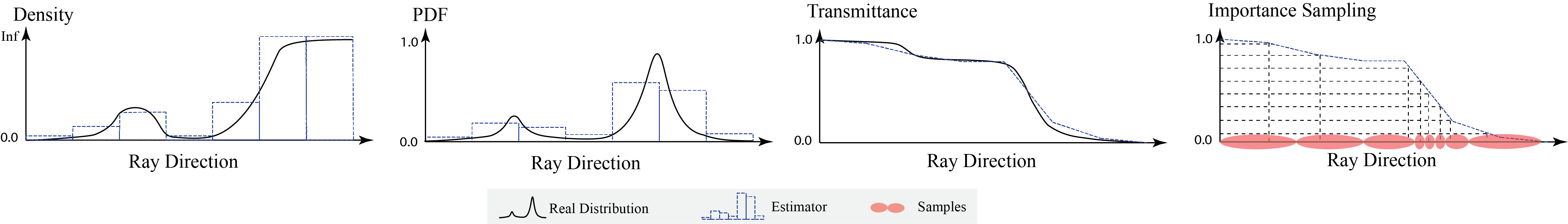
In nerfacc, this is implemented via the nerfacc.PropNetEstimator class.

Which Estimator to use?

• nerfacc.OccGridEstimator is a generally more efficient when most of the space in the scene is empty, such as in the case of NeRF-Synthetic dataset. But it still places samples within occluded areas that contribute little to the final rendering (e.g., the last sample in the above illustration).

• nerfacc.PropNetEstimator generally provide more accurate transmittance estimation, enabling samples to concentrate more on high-contribution areas (e.g., surfaces) and to be more spread out in both empty and occluded regions. Also this method works nicely on unbouned scenes as it does not require a preset bounding box of the scene. Thus datasets like Mip-NeRF 360 are better suited with this estimator.